
The Compact Reconnaissance Imaging Spectrometer for Mars (CRISM) is a Visible and Near-Infrared (VNIR) imaging spectrometer onboard Mars Reconnaissance Orbiter (MRO), in orbit since 2006. It was built and tested by the Johns Hopkins University Applied Physics Laboratory under the supervision of principal investigator Scott Murchie. The observations enable to have mineralogy information of the martian surface at a spatial resolution of ~20 to ~200 m/px.
Data description
The CRISM instrument has two acquisition modes:
The targeted mode (multiangular pointing)
The instrument tracks the targets and takes 11 hyperspectral images (544 bands from 362 to 3920 nm) at different emission angles due to the rotation of the detector at ± 70°: 10 hyperspectral images taken at different emission angles before and after the central image corresponding to the close nadir image (image #07). The 10 hyperspectral multi-angular observations are reduced to a factor 10 compared to the spatial resolution of the central image. According to the spatial resolution of the central image, four product types are associated to this acquisition mode. If the central image is sampled at 20 m/px, the associated product is a Full Resolution Targeted observation (FRT). By reducing the spatial resolution of the central image by a factor 2, the spatial resolution is set at 40 m/px and the associated products are Half Resolution Short (HRS) and Half Resolution Long (HRL) observations. An HRL sampled surface is twice as long as an HRS observation. Only the central image #07 is processed by MarsSI for the mineralogy identification. ATO observations are Along-Track Oversampled products resulting in incresing of the resolution up to 3 m/px.
| Types of targeted observations | |||
| FRT: 18 m/px | HRS: 36 m/px | HRL: 36 m/px | ATO: 3-12 m/px |
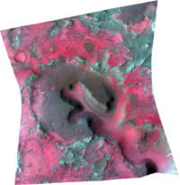 | 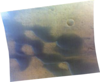 | 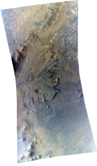 |  |
The survey mode (nadir pointing)
This mode was designed to estimate key locations for further analysis with the targeted mode as it covers wider areas and produces lower spatial resolution data than the targeted mode. The instrument acquires multispectral images using fixed pointing where the emission angle is set at 0° (with specific bands chosen over the 544 spectral bands, in order to identify principal minerals). There are different types of observations using this acquisition mode:
- Multispectral Survey (MSP): 200 m/px and 55 channels
- Hyperspectral Survey (HSP): 200 m/px and 154 channels
- Multispectral Window (MSW): 100 m/px
Downloading and processing CRISM data
- From the “Maps” tab, zoom-in on your region of interest, you can display the THEMIS mosaic for more precision, and then display the CRISM layer corresponding either to the targeted or survey mode, or You get all CRISM stamps that appear in red or pink. You can use the “Select” button to choose the stamp you desire. You can choose several stamps by clicking on several stamps, or by dragging your mouse to select adjacent stamps. You can also use the “Search” button for more options.
- To add your desired stamps to your cart click on “Add” in the “Cart” window: you can notice in the “Cart” window that different data were added: the TRDR files and the DDR files in Short (VNIR) and Long (IR) wavelength ranges, “S” and “L”. Only the “L” cubes are used in the CRISM processing and are needed for further processing in MarsSI, but you can also download the “S” cubes for your own use. Then, go to the “Workspace” tab.
- Your CRISM TRDR and DDR “L” files appear in the window “Data to process”. If not, you may already have processed them yourself, or someone else may have processed them, then they may already be in the “Data processed” window. If the data have not been processed, you will have to go download and process the TRDR and DDR cubes by clicking on the “Process” button in the “Data to process” button.
Pipeline
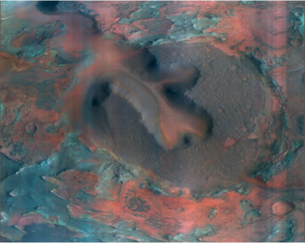
1) The TRDR cube containing the reflectance values in the infrared range will be processed using an implementation of the CAT pipeline (CRISM Analysis Tools, an add-on to IDL/ENVI available from the CRISM team (Murchie et al., 2007; Pelkey et al., 2007)). The cube will be corrected for the observation geometry (reflectance divided by the cosine of the incidence angle, available in the associated DDR cube) and for absorptions due to atmospheric CO2 using the CAT algorithm developed for CRISM based on the ‘volcano-scan’ approach (McGuire et al., 2009).
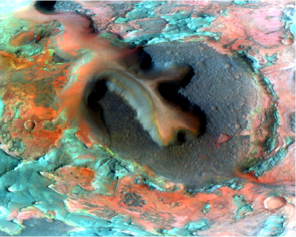
FRT00003E12_07_IF166L_TRR3_CAT_corr.img (false color composition)
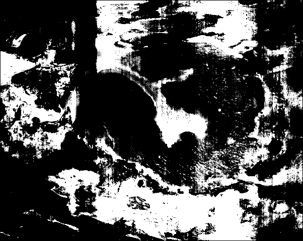
2) The targeted TRDR cube corrected for atmospheric absorption and incidence angle will then be processed through a custom pipeline to remove column-dependant noise and enhance spectral features of small spatial extent: this pipeline basically divides the whole spectral data in the cube by a median spectrum computed from half of the lines (those in the middle) of the cube, on a column-by-column basis: a procedure we dub ‘ratioing’. The output ratioed cube is dubbed medianratio. A by-product of the procedure is the creation of a transposed cube where columns and lines are switched, but which is only saved for the pipeline processing and should not be used as a standalone product. This procedure dramatically reduces detector noise (mostly column-dependant), corrects for most residual atmospheric absorptions (CO2 gas and/or water vapor/ice)and enhances small spectral features in ratioed spectra. However, there are also caveats to this ratioing procedure, such as the risk to introduce artifacts in ratioed spectra if the median spectra used for division itself was not blank but had spectral features: in such cases, the ratioed spectra will show inverted spectral features (eg., an absorption in median spectra will yield a positive peak in ratioed spectra) which will be artifacts and must not be interpreted as meaningful data. Still, for typical CRISM data, acquired over terrain with spectral features of low spatial extent (a few times smaller than the cube spatial extent), the median spectra will be nearly featureless and allow for reasonably straightforward detection of meaningful spectral features in ratioed spectra.
FRT00003E12_07_IF166L_TRR3_CAT_corr_medianratio.img (false color composition)
3) The penultimate step of the pipeline computes so-called ‘spectral parameters’ or ‘spectral criteria’ such as band depths or combination of band depths, as initially implemented in the CAT for multispectral CRISM data (Pelkey et al., 2007), or other parameters based on analysis of the shape of the spectra. We take advantage of the higher number of spectral channels in hyperspectral targeted CRISM observations compared to original CAT multispectral parameters: signal-to-noise is improved by using medians of spectral channels and specificity of criteria is improved by combining two or more criteria. The definition of a subset of the custom criteria available in MarsSI is given in Thollot et al. (2012) and the remaining can be made available on request (pending publication in a future paper). The resulting data cube, dubbed hyparam (for hyperspectral parameters), has the same spatial dimensions as the TRDR but each band in the spectral dimension contains the result of the computing of a spectral criterion designed for detection of one or several spectral features from the medianratio cube resulting from the previous step. The hyparam cube can be used in parallel with spectral data in IDL/ENVI to compare the spatial mapping of spectral criterion with actual spectra.
FRT00003E12_07_IF166L_TRR3_CAT_corr_medianratio_hyparam.img (olivine index)
4) Finally, the pipeline projects the hyparam cube (adding the _p suffix) for use in a GIS in combination with other datasets (DTMs, CTX or HiRISE, etc.).
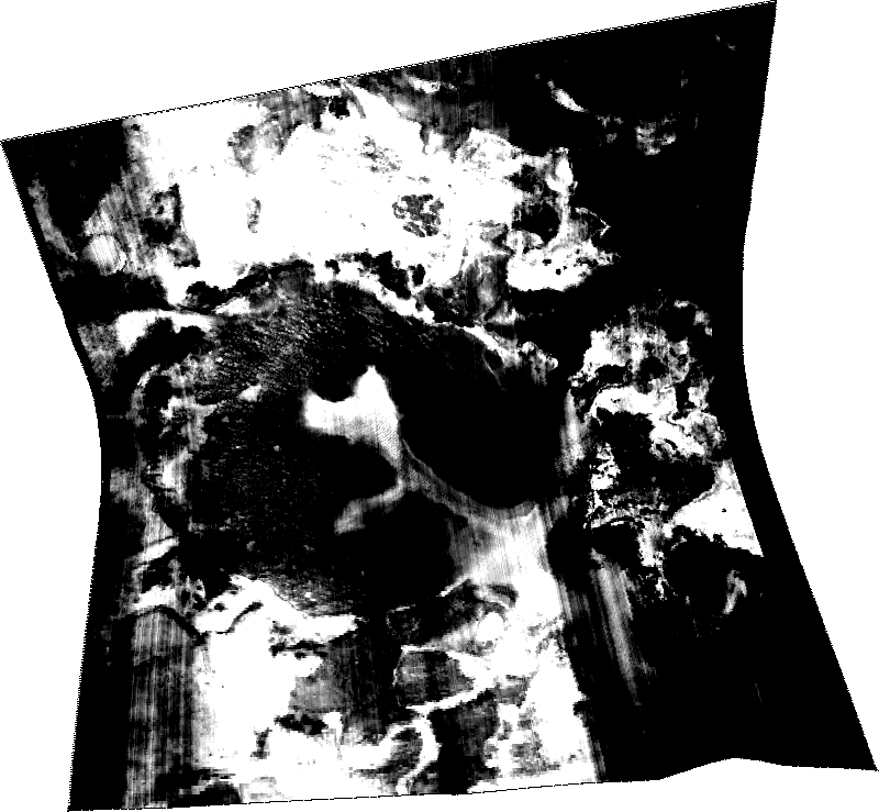
FRT00003E12_07_IF166L_TRR3_CAT_corr_medianratio_hyparam_p_equir.img (olivine index)
Data names
The CRISM naming convention is the following:
(ClassType)(ObsID)_(Counter)_(Activity)(SensorID)_(Filetype).(EXT)
ClassType: FRT, HRS, HRL, ATO, MSP, HSP, MSW, ...ObsID: observation IDCounter: image number of the targeted sequence (only the n°7 is used in MarsSI). In the survey mode, this corresponds to 1Activity: subtype of product: IF stands for reflectance data (I/F unit), DE for ancillary data (e.g. latitude, longitude, incidence, emission, phase angleSensorID: S detector (Short wavelenghts) or L (Long wavelenghts)Filetype: type of dataset: TRR3 are calibrated data cubes, DDR1 companion data cube containing the ancillary dataEXT: extension of the data (img, lbl, ...)
Ex: FRT000A82E_07_IF164L_TRR3.IMG correponds to calibrated data cube containing the reflectance data (I/F unit) in the IR range (from 1002 to 3920 nm) of the central image (corresponding to the “07” image of the targeted sequence) of an FRT observation.
Working with CRISM targeted parameters
Please consider these products with a critical eye. Despite using labels describing specific mineral (or other) detection, they are the result of spectral analysis results that are *USUALLY* typical of such minerals presence, and is presented as an evidence, but not a definitive proof of such. Be wary to not overinterpret instrument artefacts and other false positive as real results!
The hyparam cube produced by MarsSI contains computed spectral parameters. They account on each pixel for the likeness between the observation spectrum and the theoretical spectrum of a mineral specie, but can also give information on the position of absorption band, intensity of one particuliar band, etc. This cube is used to map spectral features: please keep in mind that the spectral parameters mapping does not represent mineralogical maps; to infer the true mineralogy of one location, the associated spectra (in corr or corr_medianratio cubes) should be studied carefully.
The details of how the different parameters can be used are as follows (as in april 2018):
| Band number | Parameter | Detections (non exhaustive) | Details |
| 1 | OLINDEX2 | Olivine, pyroxenes, FeMg clays | Better identifies the 1 micron olivine absorption by accounting for spectral slope. Also corrects for the false identification of olivine due to high albedo. Incorrectly maps hydrated regions as olivine-rich due to the associated decrease in reflectance beyond 2-microns. Also, like OLINDEX, this parameter falsely identifies pyroxenes as olivine. future work will be done to correct both the false identifications of hydration and pyroxene as olivine-rich. |
| 2 | BD1900R | H2O bound | Find the 1.90 micron H2O band depth |
| 3 | BD1980 | Sulfites | Find the 1.98 micron sulfite band depth |
| 4 | BD2200 | Al-OH bound | Find the 2.20 micron Al-OH band depth |
| 5 | Doub2200 | Find the 2.22 and 2.28 micron doublet band depth | |
| 6 | BD2230 | Find the 2.23 micron band depth (K. Lichtenberg) | |
| 7 | BD2500 | Carbonates | Find the 2.50 micron band depth |
| 8 | Jar_index | Jarosite | Find the 2.205-2.272 micron 'W' exact shape |
| 9 | Kaol_index | Kaolinite | Find the 2.16-2.20 asymetric kaolinite band |
| 10 | Opal_index | Opal | Find the 2.20-2.26 asymetric Opal band |
| 11 | Fe_smec_index | Fe clays | Find the 2.29 and 2.40 Fe smectite band |
| 12 | Sulf_index | Sulfates | Find the 1.94-2.0 and 2.40-2.44 non-hydrates sulfates bands |
| 13 | BD2232m | (Ferri)Copiapite / Fe sulfates | Find the 2.232 band of part. dehydr. |
| 14 | Hydr-salt_index | Bassanite, gypsum, carnallite | Find the 1.77, 1.92-1.98, 2.49 bands |
| 15 | BD2205m | Kaolinite, montmorillonite, opal | Find the 2.205 band |
| 16 | BD2205Left | Kaolinite | Find the asymetric left 2.205 band |
| 17 | BD2205Right | Opal | Find the asymetric right 2.205 band |
| 18 | BD2285m | Fe smectites | Find the 2.285 band |
| 19 | BD1922m | Hydrated minerals | Find the 1.922 band |
| 20 | BD1849m | Jarosite | Find the 1.849 band |
| 21 | BD2106m | Sulfates | Find the 2.106 band |
| 22 | BD2268m | Jarosite | Find the 2.268 band |
| 23 | BD3837m | Carbonates | Find the 3.8-3.9 band |
| 24 | POS221 | Find the exact wavelength of minimum of 2.21 band at 2.1855-2.2252 | |
| 25 | POS227 | Find the exact wavelength of minimum of 2.27 band at 2.2583-2.3046 | |
| 26 | BD1047m | Iron oxydes | Find the 1.0472 band of iron oxides relative to linear fit 1.3423-2.1261 |
| 27 | Hydr_FeMg_clay_index | Hydrated FeMg TOT clays | Find the 1.4; 1.9; 2.3; 2.4 bands |
| 28 | Si-OH_index | Hydrated glass | Find the 1.4; 1.9; 2.2 bands |
| 29 | BD2265narrow | Jarosite even within mixtures | Find the 2.265 band |
| 30 | 2205to2278 | Get 2205/2278 ratio in doublet when both bands present | |
| 31 | BD1060poly2 | Iron oxydes | Find the 1.0603 band of iron oxides relative to 2nd order polynomial fit 1.3423-1.8292-2.6021 |
| 32 | BD1080SEC | Iron oxydes | Find the 1.0800 band of iron oxides relative to 2nd order polynomial fit 1.3423,MAX(2.1525;2.2517)@2.203,2.6021 |
| 33 | Chlor_index | Chlorite | Find the 2.25 and 2.34 bands |
| 34 | BD1380-1440 | OH bound | Find the 1.4 OH band |
| 35 | POS14xx | Find the exact wavelength of minimum of 1.4 band at (1.3752)1.3818-1.4409(1.4474) | |
| 36 | BD1908m | Hydrated minerals | Find the 1.91 band |
| 37 | BD1961m | Hydrated minerals | Find the 1.96 band |
| 38 | 191to196 | Si-OH hydrated minerals | Find the 1.91/1.96 ratio in hydrated minerals, esp. Si-OH bearing |
| 39 | POS19xx | Find the exact wavelength of minimum of 1.9 band at (1.895)1.902-1.981(1.987) | |
| 40 | BD2272m_2179 | Jarosite | Find the 2.272 band of jarosite anchored at 2.18 instead of 2.09 |
| 41 | Olivine_index | Olivine | Find the 1.080, 1.257, 1.369 and 1.467 bands |
| 42 | BD1760m | Hydrated minerals | Find the 1.76 band |
| 43 | FeMg-OH | FeMg-OH bounds | Find the 2.3 and 2.4 bands |
| 44 | BD2106+2139_poly2 | Monohydrated sulfates | Find the average of 2.106 & 2.139 band of monoh. sulf. relative to 2nd order polynomial fit 1.856-2.311-2.490 |
References:
- CRISM instrument description website: http://crism.jhuapl.edu/instrument/design/overview.php
- McGuire P. C., e t al. (2009), An improvement to the volcano - scan algorithm for atmospheric correction of CRISM and OMEGA spectral data, Planet. Space Sci., 57(7), 809 - 815.
- Murchie, S., et al. (2007), Compact reconnaissance Imaging Spectrometer for Mars (CRISM) on Mars Rec onnaissance Orbiter (MRO), J. Geophys. Res., 112(E5).